How To Self Evaluate Progress On Learning Computer Science

Machine Learning for Humans, Office ii.one: Supervised Learning

The two tasks of supervised learning: regression and classification. Linear regression, loss functions, and gradient descent.

          This serial is available as a full-length e-volume!            Download here. Free for download, contributions appreciated (paypal.me/ml4h            )

How much money will we make by spending more dollars on digital advertisement? Will this loan bidder pay back the loan or not? What'due south going to happen to the stock market tomorrow?

In supervised learning bug, we kickoff with a data ready containing training examples with associated correct labels. For example, when learning to classify handwritten digits, a supervised learning algorithm takes thousands of pictures of handwritten digits along with labels containing the correct number each image represents. The algorithm volition and then learn the relationship between the images and their associated numbers, and employ that learned human relationship to classify completely new images (without labels) that the machine hasn't seen before. This is how you're able to deposit a check by taking a picture with your phone!

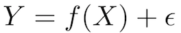
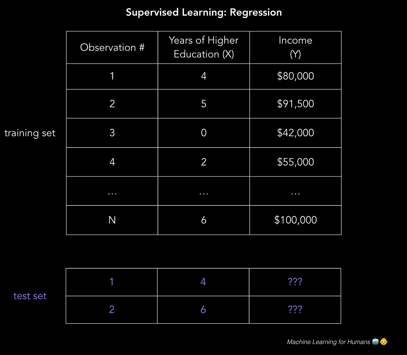
To illustrate how supervised learning works, permit'south examine the trouble of predicting annual income based on the number of years of college education someone has completed. Expressed more formally, we'd similar to build a model that approximates the relationship f between the number of years of higher education X and corresponding annual income Y.

                      X (input)            = years of college educational activity
            Y (output)            = annual income
                          f                        = function describing the relationship between X and Y
            ϵ (epsilon)            = random error term (positive or negative) with mean zip                      Regarding epsilon:                                (one) ϵ              represents                                      irreducible error                                      in the model, which is a theoretical limit around the operation of your algorithm due to inherent noise in the phenomena yous are trying to explain. For example, imagine building a model to predict the issue of a coin flip.                                (2) Incidentally, mathematician                        Paul Erdős                          referred to children as "epsilons" because in calculus (but not in stats!)            ϵ              denotes an arbitrarily pocket-sized positive quantity. Plumbing fixtures, no?

1 method for predicting income would exist to create a rigid rules-based model for how income and education are related. For example: "I'd estimate that for every additional year of college didactics, almanac income increases by $5,000."

          income = ($5,000 * years_of_education) + baseline_income                      This approach is an example of                                      engineering                                      a solution (vs.                                      learning                                      a solution, equally with the linear regression method described below).

Yous could come up with a more than complex model by including some rules well-nigh caste blazon, years of piece of work experience, schoolhouse tiers, etc. For example: "If they completed a Bachelor'south caste or higher, requite the income estimate a 1.5x multiplier."

But this kind of explicit rules-based programming doesn't work well with circuitous data. Imagine trying to pattern an image classification algorithm made of if-and so statements describing the combinations of pixel brightnesses that should exist labeled "cat" or "not cat".

Supervised machine learning solves this trouble by getting the estimator to practice the work for yous. By identifying patterns in the data, the machine is able to form heuristics. The master departure between this and human learning is that motorcar learning runs on computer hardware and is best understood through the lens of computer science and statistics, whereas human design-matching happens in a biological brain (while accomplishing the aforementioned goals).

In supervised learning, the machine attempts to acquire the relationship between income and didactics from scratch, by running labeled grooming data through a learning algorithm. This learned part tin can be used to estimate the income of people whose income Y is unknown, equally long as we have years of teaching X equally inputs. In other words, we can apply our model to the unlabeled examination information to approximate Y.

The goal of supervised learning is to predict Y equally accurately as possible when given new examples where X is known and Y is unknown. In what follows we'll explore several of the most common approaches to doing so.

The two tasks of supervised learning: regression and classification

                      Regression:            predict a continuous numerical value.            How much will that house sell for?                                Classification: assign a label.              Is this a picture of a cat or a canis familiaris?

The residual of this section will focus on regression. In Role 2.two nosotros'll dive deeper into classification methods.

Regression: predicting a continuous value

Regression predicts a continuous target variable Y. It allows you to estimate a value, such equally housing prices or human lifespan, based on input information X.

Here, target variable ways the unknown variable we care nigh predicting, and continuous means in that location aren't gaps (discontinuities) in the value that Y tin take on. A person's weight and height are continuous values. Discrete variables, on the other hand, can only take on a finite number of values — for example, the number of kids somebody has is a discrete variable.

Predicting income is a classic regression problem. Your input information X includes all relevant information about individuals in the data ready that tin can exist used to predict income, such every bit years of instruction, years of work experience, job championship, or zip lawmaking. These attributes are called features, which can be numerical (e.m. years of work experience) or categorical (e.chiliad. job title or field of report).

You'll want every bit many training observations equally possible relating these features to the target output Y, so that your model tin can learn the human relationship f betwixt X and Y.

The data is split into a preparation data set and a examination data set. The training ready has labels, so your model can learn from these labeled examples. The test gear up does not have labels, i.e. yous don't however know the value y'all're trying to predict. It's important that your model tin generalize to situations it hasn't encountered before and so that it can perform well on the test data.

                      Regression                                Y = f(X) + ϵ, where X = (x1, x2…xn)                      Training: machine learns            f            from labeled training data                      Test: automobile predicts Y from unlabeled testing data                      Note that X tin can exist a                                      tensor                                      with an any number of dimensions.            A 1D tensor is a vector (1 row, many columns), a 2D tensor is a matrix (many rows, many columns), and so you tin can have tensors with 3, 4, 5 or more dimensions (e.g. a 3D tensor with rows, columns, and depth). For a review of these terms, see the first few pages of this linear algebra review.

In our trivially simple 2d example, this could take the form of a .csv file where each row contains a person's education level and income. Add more than columns with more than features and you'll take a more circuitous, just possibly more accurate, model.

So how do we solve these problems?

How practice we build models that make accurate, useful predictions in the existent earth? Nosotros do so by using supervised learning algorithms.

Now let's become to the fun part: getting to know the algorithms. We'll explore some of the means to approach regression and classification and illustrate key auto learning concepts throughout.

Linear regression (ordinary least squares)

"Draw the line. Yes, this counts every bit machine learning."

First, we'll focus on solving the income prediction problem with linear regression, since linear models don't work well with image recognition tasks (this is the domain of deep learning, which we'll explore later).

We take our information set X, and corresponding target values Y. The goal of ordinary least squares (OLS) regression is to learn a linear model that we tin can use to predict a new y given a previously unseen x with as little error every bit possible. Nosotros want to gauge how much income someone earns based on how many years of education they received.

          X_train = [4, v, 0, ii, …, 6] # years of mail service-secondary education          Y_train = [80, 91.v, 42, 55, …, 100] # respective annual incomes, in thousands of dollars

Linear regression is a parametric method, which means it makes an assumption about the grade of the part relating X and Y (we'll cover examples of not-parametric methods later). Our model will be a function that predicts ŷ given a specific ten:

In this case, we make the explicit assumption that there is a linear human relationship between X and Y — that is, for each one-unit of measurement increase in Ten, we run into a abiding increment (or decrease) in Y.

β0 is the y-intercept and β1 is the slope of our line, i.e. how much income increases (or decreases) with one additional year of education.

Our goal is to learn the model parameters (in this case, β0 and β1) that minimize fault in the model'southward predictions.

To observe the all-time parameters:

1. Define a cost function, or loss role, that measures how inaccurate our model's predictions are.

2. Discover the parameters that minimize loss, i.east. make our model as authentic as possible.

Graphically, in two dimensions, this results in a line of all-time fit. In three dimensions, nosotros would draw a plane, and and so on with higher-dimensional hyperplanes.

                      A note on dimensionality: our example is two-dimensional for simplicity, only you lot'll typically have more features (ten'southward) and coefficients (betas) in your model, e.g. when calculation more relevant variables to improve the accuracy of your model predictions. The same principles generalize to higher dimensions, though things go much harder to visualize across 3 dimensions.

Mathematically, we look at the departure betwixt each real information point (y) and our model'southward prediction (ŷ). Foursquare these differences to avoid negative numbers and penalize larger differences, and so add them up and take the average. This is a measure of how well our data fits the line.

n = # of observations. Using ii*n instead of n makes the math work out more cleanly when taking the derivative to minimize loss, though some stats people say this is blasphemy. When y'all start having opinions on this kind of stuff, you'll know you are all the fashion in the rabbit hole.

For a simple problem similar this, we can compute a closed course solution using calculus to notice the optimal beta parameters that minimize our loss office. But as a cost function grows in complexity, finding a closed form solution with calculus is no longer feasible. This is the motivation for an iterative approach called gradient descent, which allows us to minimize a complex loss function.

Gradient descent: learn the parameters

"Put on a blindfold, take a step downhill. Y'all've found the bottom when you have nowhere to go just up."

Gradient descent will come up over and again, peculiarly in neural networks. Machine learning libraries similar scikit-learn and TensorFlow use information technology in the background everywhere, and then information technology's worth understanding the details.

The goal of gradient descent is to discover the minimum of our model'southward loss function by iteratively getting a meliorate and better approximation of it.

Imagine yourself walking through a valley with a blindfold on. Your goal is to detect the bottom of the valley. How would yous do it?

A reasonable arroyo would be to touch the ground around you and move in whichever direction the ground is sloping down about steeply. Take a step and repeat the same process continually until the footing is flat. Then yous know you've reached the bottom of a valley; if yous movement in any direction from where y'all are, you lot'll end upwards at the same superlative or further uphill.

Going back to mathematics, the ground becomes our loss function, and the elevation at the bottom of the valley is the minimum of that office.

Let'due south take a await at the loss function we saw in regression:

We run across that this is actually a function of two variables: β0 and β1. All the rest of the variables are adamant, since 10, Y, and north are given during training. Nosotros want to try to minimize this function.

The function is f(β0,β1)=z. To brainstorm gradient descent, you make some guess of the parameters β0 and β1 that minimize the part.

Next, you detect the partial derivatives of the loss function with respect to each beta parameter: [dz/dβ0, dz/dβ1]. A partial derivative indicates how much total loss is increased or decreased if yous increase β0 or β1 by a very pocket-size amount.

Put another way, how much would increasing your judge of annual income bold nada higher educational activity (β0) increment the loss (i.e. inaccuracy) of your model? You want to become in the reverse direction then that yous end up walking downhill and minimizing loss.

Similarly, if yous increase your estimate of how much each incremental year of instruction affects income (βane), how much does this increase loss (z)? If the partial derivative dz/β1 is a negative number, then increasing β1 is proficient because it will reduce total loss. If information technology's a positive number, you lot want to decrease β1. If it'due south zippo, don't change β1 considering it means you've reached an optimum.

Go on doing that until you reach the lesser, i.due east. the algorithm converged and loss has been minimized. In that location are lots of tricks and exceptional cases beyond the scope of this series, simply generally, this is how you notice the optimal parameters for your parametric model.

Overfitting

Overfitting: "Sherlock, your caption of what just happened is as well specific to the situation." Regularization: "Don't overcomplicate things, Sherlock. I'll punch you for every actress discussion." Hyperparameter (λ): "Hither'due south the force with which I will punch you for every extra word."

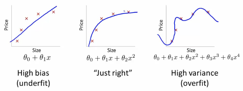
A mutual problem in machine learning is overfitting: learning a function that perfectly explains the training information that the model learned from, merely doesn't generalize well to unseen test information. Overfitting happens when a model overlearns from the training data to the point that it starts picking up idiosyncrasies that aren't representative of patterns in the real world. This becomes especially problematic every bit you make your model increasingly complex. Underfitting is a related outcome where your model is not complex enough to capture the underlying trend in the data.

                      Bias-Variance Tradeoff                                Bias            is the corporeality of error introduced by approximating existent-world phenomena with a simplified model.                      Variance            is how much your model's exam fault changes based on variation in the grooming data. It reflects the model's sensitivity to the idiosyncrasies of the data set up it was trained on.          As a model increases in complexity and information technology becomes more wiggly (flexible), its bias decreases (it does a good job of explaining the preparation data), but variance increases (it doesn't generalize also).            Ultimately, in society to accept a proficient model, you need 1 with low bias              and              low variance.

Source: Coursera's ML course, taught by Andrew Ng

Recollect that the but thing we care about is how the model performs on test data. Y'all want to predict which emails will be marked as spam earlier they're marked, not just build a model that is 100% accurate at reclassifying the emails it used to build itself in the starting time identify. Hindsight is 20/20 — the real question is whether the lessons learned will help in the futurity.

The model on the correct has nada loss for the training data considering it perfectly fits every data point. Only the lesson doesn't generalize. Information technology would do a horrible task at explaining a new data point that isn't yet on the line.

Two means to combat overfitting:

one. Apply more training information. The more yous have, the harder it is to overfit the data by learning as well much from any single training example.

2. Employ regularization. Add in a penalty in the loss part for edifice a model that assigns too much explanatory power to whatsoever one characteristic or allows too many features to exist taken into account.

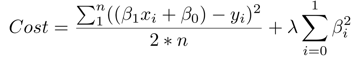
The first piece of the sum to a higher place is our normal cost function. The second piece is a regularization term that adds a penalisation for big beta coefficients that give also much explanatory power to any specific feature. With these 2 elements in identify, the cost part now balances between two priorities: explaining the training data and preventing that caption from becoming overly specific.

The lambda coefficient of the regularization term in the cost function is a hyperparameter: a general setting of your model that tin can exist increased or decreased (i.e. tuned) in social club to improve performance. A higher lambda value will more harshly penalize large beta coefficients that could lead to potential overfitting. To determine the best value of lambda, yous'd utilize a method called cross-validation which involves belongings out a portion of the training data during training, and then seeing how well your model explains the held-out portion. We'll get over this in more depth

Woo! We made it.

Here's what nosotros covered in this section:

How supervised machine learning enables computers to learn from labeled grooming data without being explicitly programmed
The tasks of supervised learning: regression and classification
Linear regression, a bread-and-butter parametric algorithm
Learning parameters with gradient descent
Overfitting and regularization

In the adjacent section — Role 2.2: Supervised Learning Two — we'll talk most ii foundational methods of classification: logistic regression and support vector machines.

Practice materials & further reading

2.1a — Linear regression

For a more thorough treatment of linear regression, read chapters ane–3 of An Introduction to Statistical Learning . The book is available for gratuitous online and is an excellent resource for understanding auto learning concepts with accompanying exercises.

For more practice:

Play with the Boston Housing dataset . You tin can either utilise software with nice GUIs like Minitab and Excel or do it the hard (but more rewarding) style with Python or R .
Effort your hand at a Kaggle challenge, eastward.g. housing price prediction , and come across how others approached the trouble after attempting it yourself.

2.1b — Implementing gradient descent

To really implement gradient descent in Python, check out this tutorial . And here is a more mathematically rigorous clarification of the same concepts.

In do, you'll rarely need to implement slope descent from scratch, just understanding how it works backside the scenes will permit you to apply information technology more than effectively and understand why things break when they do.